Fájl:Newton iteration.png

Az oldal más nyelven nem érhető el.
A Wikipédiából, a szabad enciklopédiából

Eredeti fájl(2 406 × 1 978 képpont, fájlméret: 55 KB, MIME-típus: image/png)

Összefoglaló

Ez a kép elérhető vektorgrafikus (SVG) változatban is. Ha jobb minőségű, azt használd e helyett a raszterkép helyett.

File:Newton iteration.png → File:Newton iteration.svg

A vektorgrafikáról a Help:SVG oldalon találsz információkat.
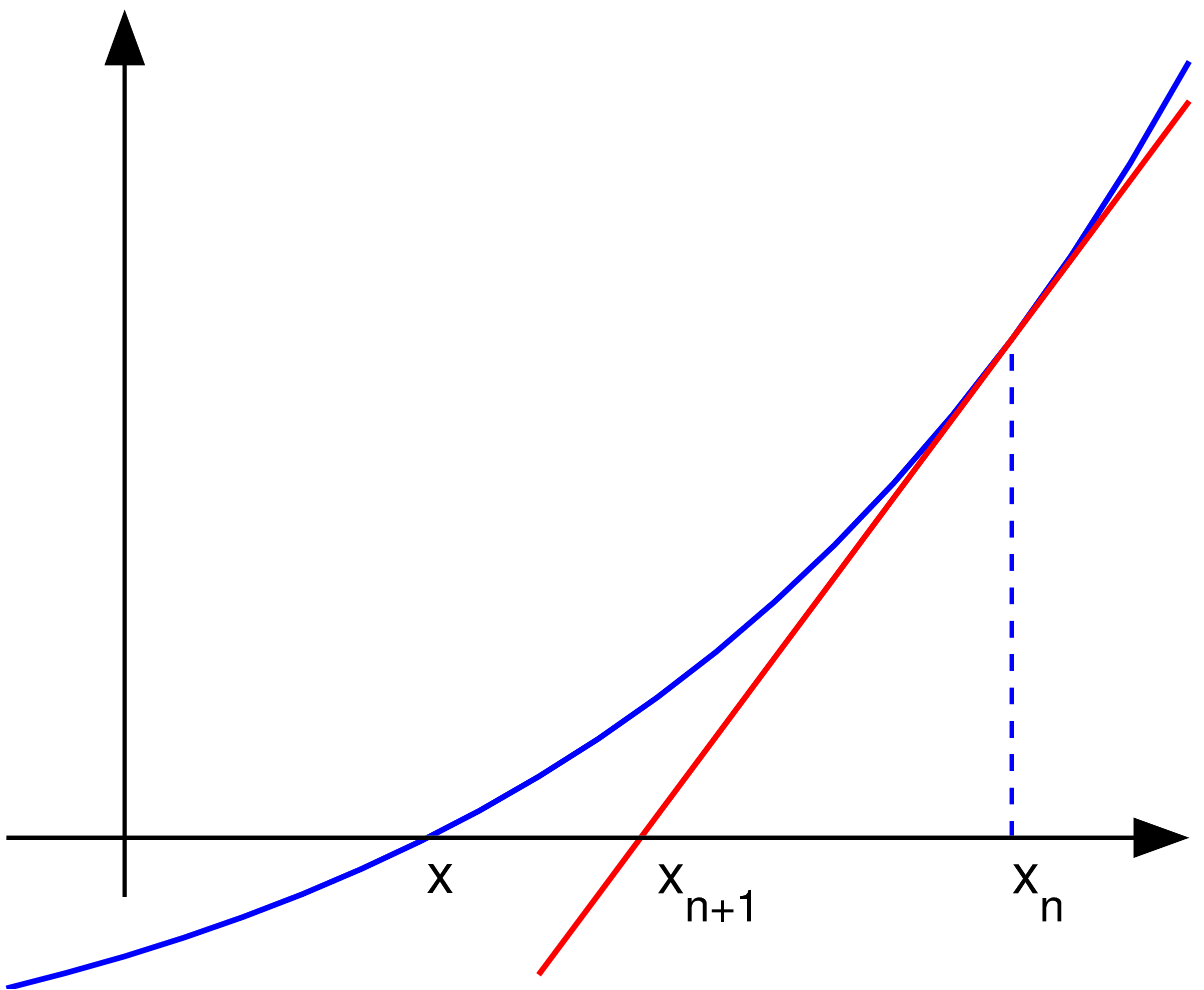
Más nyelveken
Alemannisch  Bahasa Indonesia  Bahasa Melayu  British English  català  čeština  dansk  Deutsch  eesti  English  español  Esperanto  euskara  français  Frysk  galego  hrvatski  Ido  italiano  lietuvių  magyar  Nederlands  norsk bokmål  norsk nynorsk  occitan  Plattdüütsch  polski  português  português do Brasil  română  Scots  sicilianu  slovenčina  slovenščina  suomi  svenska  Tiếng Việt  Türkçe  vèneto  Ελληνικά  беларуская (тарашкевіца)  български  македонски  нохчийн  русский  српски / srpski  татарча/tatarça  українська  ქართული  հայերեն  বাংলা  தமிழ்  മലയാളം  ไทย  한국어  日本語  简体中文  繁體中文  עברית  العربية  فارسی  +/−
Az új SVG kép

Leírás Uploader graphed this with en:MATLAB (Illustration of en:Newton's method)
Dátum 2004. november 22. (first version); 2004-11-23 (last version)
Forrás Áthozva az en.wikipedia projektből a Commonsba.
Szerző Olegalexandrov a(z) angol Wikipédia projektből
PNG kód
InfoField
 
Ez PNG számítógépes grafika MATLAB segítségével készült
Forráskód
InfoField

MATLAB code

(Newton iteration)
% illustration of Newton's method for finding a zero of a function

function main ()
   
a=-1; b=1;   % interval endpoints
fs=20;       % text font size

% arrows settings
thickness1=2; thickness2=1.5; arrowsize=0.1; arrow_type=1;
angle=20; % in degrees

h=0.1;  % grid size
X=a:h:b; % points on the x axis
f=inline('exp(x)/1.5-0.5');   % function to plot
g=inline('exp(x)/1.5');       % derivative of f
x0=0.7; y0=f(x0);             % point at which to draw the tangent line 
m=g(x0);
Y=f(X);                       % points on the function to plot
XT=-0.1:h:b; YT=y0+(XT-x0)*m; % tangent line

% prepare the screen
clf; hold on; axis equal; axis off

% plot the graph and the tangent lines
plot(X, Y, 'linewidth', thickness1)
plot(XT, YT, 'r', 'linewidth', thickness1)
plot([x0 x0], [0, y0], '--', 'linewidth', thickness2)

% axes
small=0.2;
arrow([a 0], [b, 0], thickness2, arrowsize, angle, arrow_type, [0, 0, 0])
arrow([a+small, -0.1], [a+small, 1.4], thickness2, arrowsize, angle, arrow_type, [0, 0, 0])

% text
H=text(-0.29, -0.06,  'x'); set(H, 'fontsize', fs)
H=text(0.1, -0.1,  'x_{n+1}'); set(H, 'fontsize', fs)
H=text(0.7, -0.1,  'x_{n}'); set(H, 'fontsize', fs)

% save to disk
saveas(gcf, 'newton_iteration.eps', 'psc2')

function arrow(start, stop, thickness, arrow_size, sharpness, arrow_type, color)

% Function arguments:
% start, stop:  start and end coordinates of arrow, vectors of size 2
% thickness:    thickness of arrow stick
% arrow_size:   the size of the two sides of the angle in this picture ->
% sharpness:    angle between the arrow stick and arrow side, in degrees
% arrow_type:   1 for filled arrow, otherwise the arrow will be just two segments
% color:        arrow color, a vector of length three with values in [0, 1]

% convert to complex numbers
   i=sqrt(-1);
   start=start(1)+i*start(2); stop=stop(1)+i*stop(2);
   rotate_angle=exp(i*pi*sharpness/180);

% points making up the arrow tip (besides the "stop" point)
   point1 = stop - (arrow_size*rotate_angle)*(stop-start)/abs(stop-start);
   point2 = stop - (arrow_size/rotate_angle)*(stop-start)/abs(stop-start);

   if arrow_type==1 % filled arrow

      % plot the stick, but not till the end, looks bad
      t=0.5*arrow_size*cos(pi*sharpness/180)/abs(stop-start); stop1=t*start+(1-t)*stop;
      plot(real([start, stop1]), imag([start, stop1]), 'LineWidth', thickness, 'Color', color);

      % fill the arrow
      H=fill(real([stop, point1, point2]), imag([stop, point1, point2]), color);
      set(H, 'EdgeColor', 'none')

   else % two-segment arrow
      plot(real([start, stop]), imag([start, stop]),   'LineWidth', thickness, 'Color', color);
      plot(real([stop, point1]), imag([stop, point1]), 'LineWidth', thickness, 'Color', color);
      plot(real([stop, point2]), imag([stop, point2]), 'LineWidth', thickness, 'Color', color);
   end

Licenc

Public domain Olegalexandrov a(z) angol Wikipédia projektből, a mű szerzője művét közkinccsé nyilvánította. Ez a világ minden részén érvényes.
Egyes országokban ez jogilag nem lehetséges. Ha így van, akkor:
Olegalexandrov jogot ad bárkinek, hogy bármilyen célból, feltétel nélkül használhassa ezt a fájlt, kivéve a törvény által kötelezően előírt feltételeket.


Eredeti feltöltési napló

Az eredeti leírólap itt volt. Az itt következő felhasználónevek az en.wikipedia projektre hivatkoznak.
  • 2004-11-23 19:55 Olegalexandrov 405×340×8 (14290 bytes) Scaled down the picture of Newton's method
  • 2004-11-22 21:34 Olegalexandrov 509×406×8 (16510 bytes) I graphed this with Matlab (Illustration of Newton's method) {{PD}}

Képaláírások

Adj meg egy egysoros magyarázatot arról, hogy mit mutat be ez a fájl

A fájl által ábrázolt elemek

mű tárgya

Fájltörténet

Kattints egy időpontra, hogy a fájl akkori állapotát láthasd.

Dátum/időBélyegképFelbontásFeltöltőMegjegyzés
aktuális2007. május 25., 05:23Bélyegkép a 2007. május 25., 05:23-kori változatról2 406 × 1 978 (55 KB)Oleg Alexandrov{{Information |Description=Uploader graphed this with en:MATLAB (Illustration of en:Newton's method) ==Source code== <pre> <nowiki> % illustration of Newton's method for finding a zero of a function function main () a=-1; b=1; % interva
2005. június 13., 01:11Bélyegkép a 2005. június 13., 01:11-kori változatról405 × 340 (6 KB)Everlongoptimized for smaller file size
2005. január 18., 01:06Bélyegkép a 2005. január 18., 01:06-kori változatról405 × 340 (14 KB)Andreas Ipp~commonswiki{{PD}}: Original author graphed this with MATLAB (Illustration of Newton's method), from Wikipedia.

Ezt a fájlt nem használja egyetlen lap sem.

Globális fájlhasználat

A következő wikik használják ezt a fájlt: